Chapter 7 Simple Linear Regression
A model for a continuous response variable and a continuous explanatory variable, between which a linear relationship is assumed. The data-generating process is assumed to follow a normal distribution, given the effect of the explanatory variable.
7.1 Overview
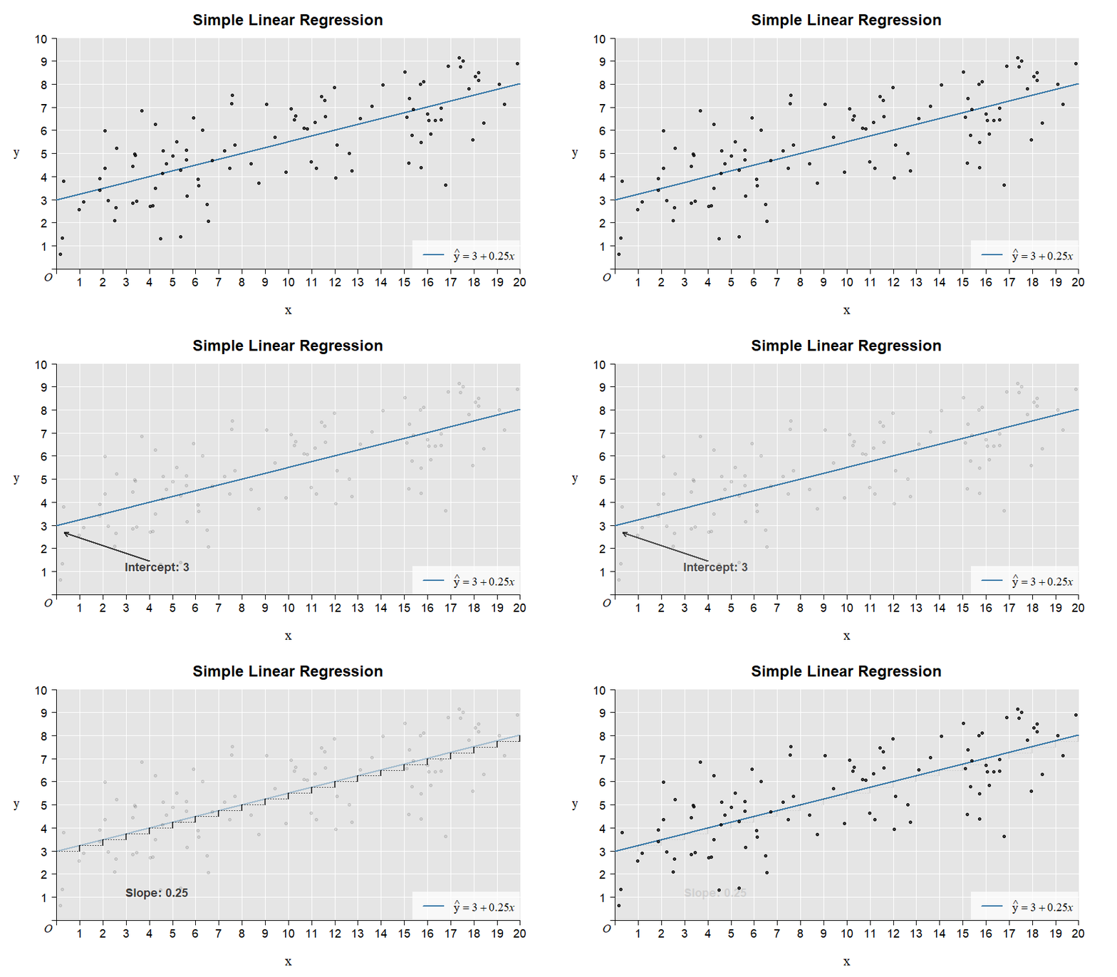
Here is the illustration of the intercept and slope:

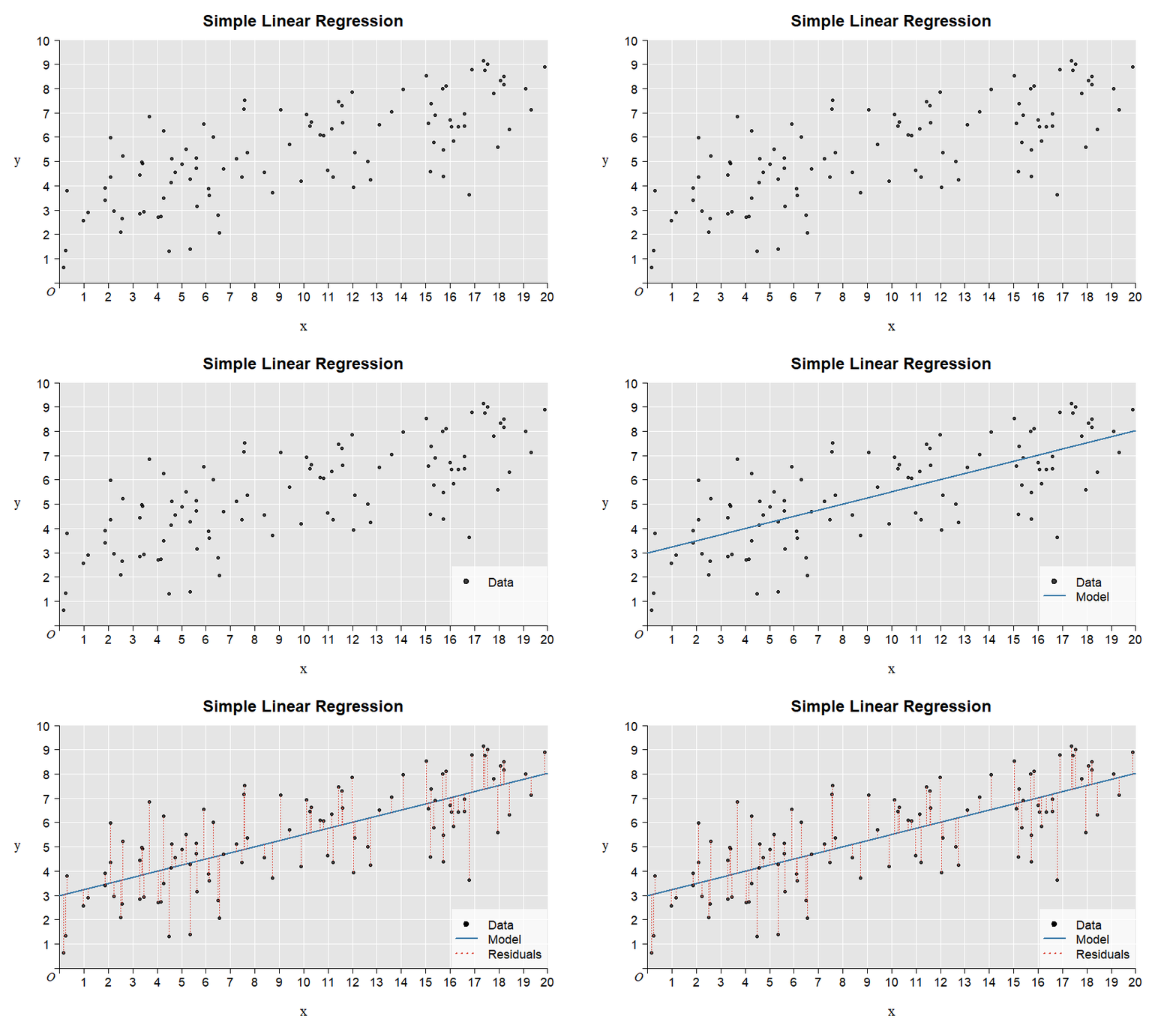
Here is the illustration of the residuals:

7.1.1 Summary of the example in the video
1. Enter your data: (you can use other methods)
BMI <- c(18.4, 31.2, 22.7, 21.6, 27.0, 27.1, 17.5, 20.9, 26.6, 27.6,
         25.2, 25.1, 25.7, 26.1, 32.4, 31.6, 17.2, 29.1, 32.9, 20.6)
BFP <- c(18.9, 26.0, 22.1, 13.2, 17.3, 22.9, 13.9, 29.2, 35.4, 20.6,
         30.3, 32.1, 27.2, 28.2, 38.2, 31.3, 15.2, 36.7, 24.8, 18.3)
DF  <- data.frame(BMI, BFP)
2. Plot your data
plot(BFP ~ BMI, data = DF)3. Fit a simple linear model:
LM <- lm(BFP ~ BMI, data = DF) 4. Perform visual diagnostics:
require("car")         # Install if missing
par(mfrow = c(2, 2))   # Plot in a 2x2 grid
plot(LM, which = 1)    # Residuals vs fitted
qqPlot(LM, reps = 1e4) # use plot(LM, which = 2 in case of errors)
plot(LM, which = 3)    # Scale-location
plot(LM, which = 5)    # Cook's distance vs leverage
par(mfrow = c(1, 1))   # Restore the default
5. Check the regression table:
summary(LM)6. Plot your model and write a conclusion about it:
plot(BFP ~ BMI, data = DF)
lines(coef(LM))
text(32.5, 12.5, bquote(R^2 == .(round(summary(LM)$r.squared, 3))))
7. You could add a prediction interval:
plot(BFP ~ BMI, DF)
x_values  <- seq(15, 35, 0.1) # 15, 15.1, 15.2, ..., 35
newdata   <- data.frame(BMI = x_values)
y_predict <- predict(LM, newdata, interval = "predict", level = 0.95)
lines(y_predict[, 1] ~ x_values)          # Regression line
lines(y_predict[, 2] ~ x_values, lty = 2) # Lower bound
lines(y_predict[, 3] ~ x_values, lty = 2) # Upper bound7.2 Step-by-Step Walkthrough
Here is a comprehensive tutorial by Dr. H.G.J. van Mil, using simulated data:
You can watch the video while trying to reproduce the steps. You can change some of the simulation input if you like:
Simulation code:
set.seed(635)
n         <- 20
Intercept <- 220
Slope     <- 3.5
Phosphate <- runif(n, 0, 10)
Residuals <- rnorm(n, 0, 3)
Biomass   <- Intercept + Slope * Phosphate + Residuals
SimDat    <- data.frame(Biomass, Phosphate)
From there on you will have an object in your workspace called SimDat that contains the simulated data set. You can use it to follow the steps shown in Harald’s video.
7.3 Model Diagnostics
7.3.1 Exercises
Below is a famous standard data set in R on the distance until a car has stopped completely from the moment it starts braking.4 Its variables are:
dist: numeric stopping distance (ft)speed: numeric speed (mph)
data(cars)Fit a simple linear model and perform visual diagnostics. Is this an appropriate model? Why?
Fit the following model with a square-root transformation of the outcome and compare the diagnostic plots. Which do you think is better and why?
LM2 <- lm(sqrt(dist) ~ speed, cars)- Complete the analysis using the example analysis. Report a conclusion.
7.4 Transformation
In yesterday’s rice and fruitfly data we observed that the assumption of homoscedasticity is not correct for these data. In the lecture on model diagnostics, transformation was briefly discussed. In this screencast, Harald discusses transformation in the context of the fruitfly data:
Ezekiel, M. (1930) Methods of Correlation Analysis. Wiley.↩︎