Chapter 4 Statistical Tests
How do you perform basic comparisons of samples? How do you calculate test statistics, what do they mean, and when is something significant? This chapter covers everything you need to know about basic significance tests for GRS, including the \(t\)-test, \(\chi^2\)-test, and multiple testing correction.
4.1 T-Test
A test for comparing two group means. The data-generating process is assumed to follow a normal distribution, given the group.
4.1.1 Choosing the right \(t\)-test
Watch part 1 of the \(t\)-test lecture and answer the questions below.
4.1.2 Exercises
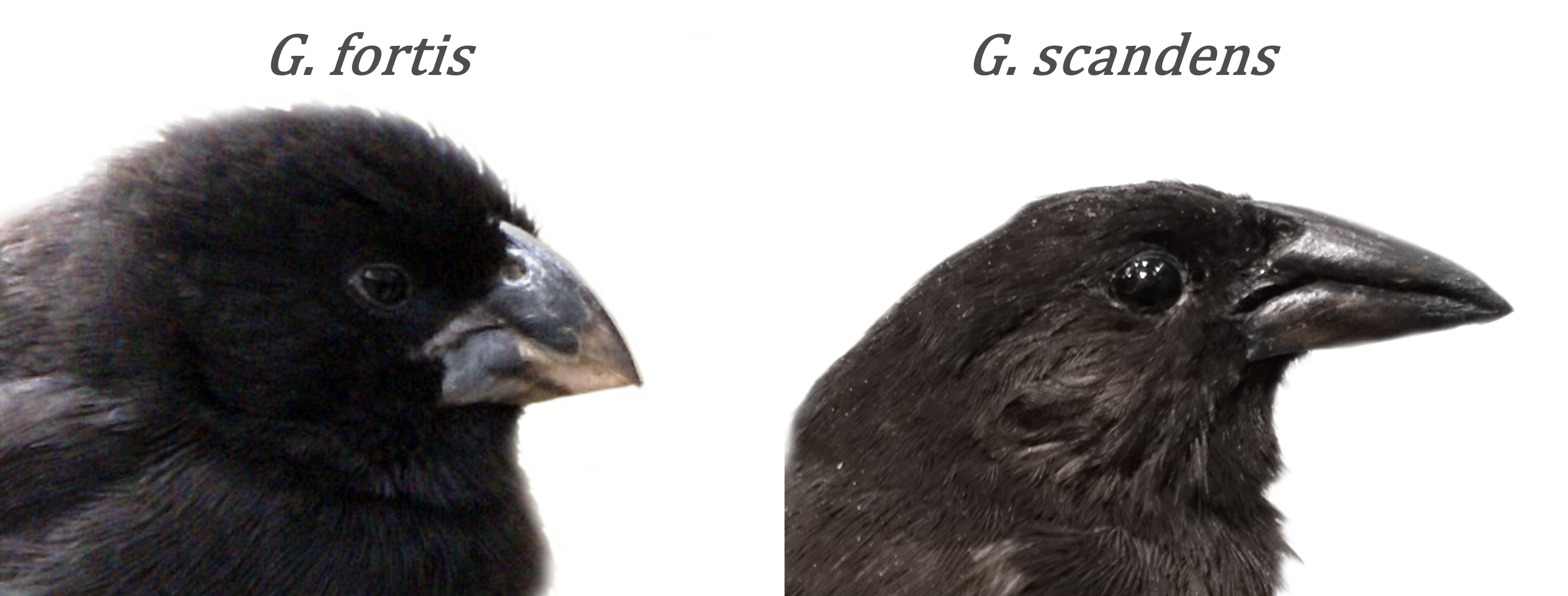
- Suppose you measured the beak dimensions (length, depth) of three Geospiza fortis and three Geospiza scandens finches. Copy the code below to enter the example data into R:
fortis_length   <- c(11.00, 10.60, 11.43)
fortis_depth    <- c(9.70, 9.30, 10.28)
scandens_length <- c(12.90, 14.20, 14.00)
scandens_depth <- c(7.90, 9.10, 8.80)- Is there a significant difference in mean beak length at \(\alpha = 0.05\)? Use an appropriate \(t\)-test.
- Is there a significant difference in mean beak depth at \(\alpha = 0.05\)? Use an appropriate \(t\)-test.
If you use a Wilcoxon test instead of a \(t\)-test, how does this affect your conclusion?
Suppose you measure three juvenile G. fortis finches, tag them, and then measure them again once they reach adulthood:
juvenile_length <- c(8.69, 7.69, 8.11)
juvenile_depth  <- c(9.44, 7.22, 8.38)
adult_length    <- c(11.50, 9.70, 10.40)
adult_depth <- c(9.50, 8.00, 8.80)- Is there a significant difference in mean beak length at \(\alpha = 0.05\)? Use an appropriate \(t\)-test.
- Is there a significant difference in mean beak depth at \(\alpha = 0.05\)? Use an appropriate \(t\)-test.
4.1.3 Understanding how the \(t\)-test works
Watch part 2 of the \(t\)-test lecture and answer the questions below.
4.1.4 Exercises
Interpreting output is an important part of the exam. The questions on the exam will usually be no harder than this, so if you get these right, your understanding of the subject matter is sufficient.
(If you want to review specific parts of the video, there are chapters if you watch it in a separate window.)
- Below is the (partial) output of a \(t\)-test. What kind of \(t\)-test is this?
t = -1.8608, df = 17.776, p-value = 0.07939
alternative hypothesis: true difference in means is not equal to 0
95 percent confidence interval:
 -3.3654832  0.2054832
sample estimates:
mean in group 1 mean in group 2
           0.75            2.33
Use the output shown above to determine what the standard error (\(\text{SE}\)) was.
Below is the output of another \(t\)-test on the same data. What kind of \(t\)-test was used here?
t = -1.8608, df = 17.776, p-value = 0.0397
alternative hypothesis: true difference in means is less than 0
95 percent confidence interval:
       -Inf -0.1066185
sample estimates:
mean in group 1 mean in group 2
           0.75            2.33
Compare the \(p\)-value of the first and second \(t\)-test. What do you notice?
What was the total sample size of the data used in the \(t\)-test below?
t = -4.9005, df = 38, p-value = 1.811e-05
alternative hypothesis: true difference in means is not equal to 0
95 percent confidence interval:
 -8.994387 -3.735613
sample estimates:
mean in group 1 mean in group 2
         19.735          26.100
(hard) Using your answer from (5) and the output, can you calculate the standard deviation (\(s\))? You may assume equal sample sizes. (If you get stuck, have a look here.)
(hard) A set of extra exercises can be downloaded here and its required data sets here.
(If you can’t knit, click here for a PDF version of the exercises.)
4.2 Chi-Squared Test
A test for comparing observed to expected frequencies (counts). Can also be used for contingency tables.
4.2.2 Exercises
Suppose a vaccine is reported to prevent \(95\%\) of virus infections in healthy adults. The vaccine is given to \(1000\) healthy adults, all of which are expected to be exposed to the virus. If \(63\) individuals end up being infected, is there a significant deviation from the reported effectiveness at \(\alpha = 0.05\)?
Below is a \(2 \times 2\) contingency table:
| male | female | |
|---|---|---|
| left-handed | 59 | 455 |
| right-handed | 40 | 479 |
- With \(\alpha = 0.05\), is there a difference in the \(\text{male}:\text{female}\) ratio of left and right-handed individuals?
- For larger contingency tables, a \(p\)-value alone does not quite paint the picture of what is going on. This is why there have been quite a few attempts to make visual summaries of categorical data. One such example is a mosaic plot. The code below generates a mosaic plot for the hair and eye color frequencies of \(592\) individuals.1 Copy the code to R and run it. Can you tell which combinations are less common in females than in males?
mosaicplot(HairEyeColor)4.3 Multiple Testing
If a study involves testing more than one hypothesis, then there is an increased chance of a false positive.
4.3.2 Exercises
- Suppose a paper compares \(10\) different diets with paired \(t\)-tests (before and after), to find out which diets result in a significant reduction in fat mass. If a level of significance \(\alpha = 0.05\) is used and no multiple testing correction is applied, what is the chance of at least one false positive?
- Suppose the results of the paper described in the previous question are the ten \(p\)-values shown below. Copy the code to your R markdown file and answer the following questions:
pvalues <- c(`diet 1`  = 0.06936,
             `diet 2`  = 0.81778,
             `diet 3`  = 0.94262,
             `diet 4`  = 0.26938,
             `diet 5`  = 0.16935,
             `diet 6`  = 0.03390,
             `diet 7`  = 0.17879,
             `diet 8`  = 0.64167,
             `diet 9`  = 0.02288,
`diet 10` = 0.00832)- Which diets have a significant effect after Bonferroni correction?
- Which diets have a significant effect after FDR correction?
- Why are some \(p\)-values equal to \(1\) after correction?
- There have been many criticisms of the over-reliance of scientific papers on \(p\)-values. This is in part because there are many incorrect interpretations being used in papers, and in part because problems like multiple testing, stopping rules and stepwise regression are often left unaddressed. This is one of the major reasons for the ongoing reproducibility crisis.
- Which of the following interpretations are incorrect? The \(p\)-value is:
- The chance of a false positive;
- The chance that the null-hypothesis is false;
- The chance that the null-hypothesis is correct;
- The chance that the alternative hypothesis is false;
- \(1\) minus the chance that the alternative hypothesis is correct;
- The probability that the results arose by chance;
- The chance that the test statistic is this large, or larger, if the null-hypothesis were correct;
- If the null-hypothesis were true, and the experiment were repeated a large number of times, then the \(p\)-value is the expected proportion of experiments with this larger, or larger a test statistic.
- A solution to the reproducibility crisis proposed by some groups is to lower the commonly used standard of \(\alpha = 0.05\) to some lower value, like \(\alpha = 0.005\). Why is this solution problematic?
- What would be a better solution?
- Below is a comic from xkcd.com. What is meant by this comic?

Snee, R. D. (1974): Graphical display of two-way contingency tables. The American Statistician, 28, 9–12. doi: 10.2307/2683520.↩︎